For modeling the oceans and atmosphere, there are three strategies for simulating the fluid in question. Indeed, these ideas are used for fluids besides the oceans and atmosphere, but they are discussed here only in the context of geophysical fluids.
The three techniques are:
- Direct Numerical Simulation (DNS)
- Reynolds-Averaged Navier-Stokes (RANS)
- Large-Eddy Simulation (LES)
Although the latter is the focus of this website, discussion of the first two elements will provide a more clear picture of how LES fits into the picture by providing context and comparison.
Direct Numerical Simulation
The DNS method opts to completely simulate the fluid flow from the largest scales all the way down to the length-scale at which molecular dissipation becomes the dominant regime. Depicted in the figure below, the energy spectrum corresponding to eddies above the dissipative scale (left of vertical line) are not modeled; the basic physics fully resolves the turbulence to those levels, and the molecular viscosity handles those which are dissipative (right of the vertical).

For even moderate scale problems in general, this is infeasible. The number of grid-points necessary to completely resolve features of this magnitude scales as $O(Re^{9/4})$. If one were to model a $1 km^3$ region of the ocean where a typical velocity scale is $O(1m/s)$, the computational domain would need to consist of $$Re^{9/4}=(UL/\nu)^{9/4}\approx (1m/s\cdot 10^3m\;/\;10^{-6}m^2/s)^{9/4}=O(10^{9/2})$$ grid-points. For real-world geophysical models, a 10km-resolution grid is often used simulation of areas $O(10^3km^2)$, so the large value $Re=O(10^{20})$ [1] requires a DNS computational grid with $O(10^{45})$ grid-points to resolve all turbulent structures to the dissipative limit. For this reason, the RANS and LES methods attempt to $indirectly$ represent the effects of turbulence as deviations from the background flow, albeit in different ways.
Reynolds-Averaged Navier-Stokes (RANS)
As a numerical scheme, the RANS method (sometimes interpreted as "Reynolds-Averaged Numerical Scheme") is most often used to find steady-state flows on a domain, although further description of unsteady formulations are readily found in [1,3]. The main idea here is to represent the velocity as $\mathbf{u}(x,t)=\overline{\mathbf{u}}(x)+\mathbf{u}\!'(x,t)$ (where $\mathbf{u'}$ is the turbulent component), and to fully simulate the average background flow independent of time. Graphically, this parametrization of the energy cascade can be represented by the following from [3]:

The RANS scheme uses a temporal average of the form \[ \overline{\mathbf{u}}(x)=\lim_{T\to\infty}\frac{1}{T}\int_0^T \mathbf{u}(x,t)dt.\] Note again that the background flow is defined as an average in time and corresponds to a steady state. The corresponding solution then represents a statistical average of the flow, rather than the flow itself even in the time-dependent case [3]. Although no single small-scale turbulent structures are not resolved, their effects and interactions with the resolved features are represented statistically [3]. The resulting numerics methods based on this simplification are acheived with significantly less computational effort, at the expense of great simplification.
Large-Eddy Simulation (LES)
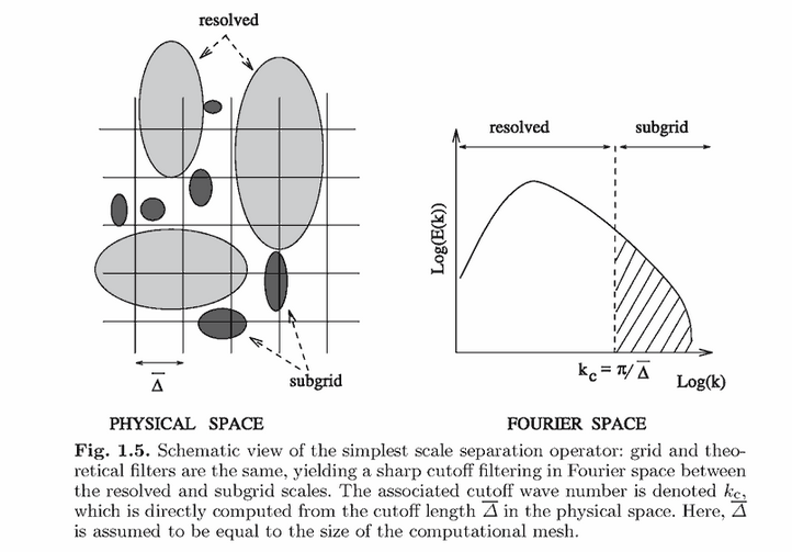
In stark contrast to the RANS methodology, the LES strategy aims to resolve eddy dynamics and turbulent energy over a particular range of scales [1,6]. This is accomplished on a domain in $ℝ^d$ by applying a spatial filter to the velocity:
\[ \overline{\mathbf{u}}\!(x,t)=g(x)*\mathbf{u}\!(x,t)=\int_{ℝ^d} g(x-x')\mathbf{u}\!(x',t)\, dx'\]
where the choice of the filter $g(x)$ determines the length scales and turbulent energies resolved by the scheme. After filtering, the NSE are rederived in terms of $\overline{\mathbf{u}}$ and the fluctuations $\mathbf{u}-\overline{\mathbf{u}}$ [1]. Upon numerical solution of the new equations, this gives a solution which hopes to reflect the filter-specified \overline{\mathbf{u}} and parametrizes the rest. Which scales are filtered (choice of $g$) and how the unfiltered scales are dealt with (sub-grid model) is technical and still an active area of research.

The choices of filter $g$ is of utmost importance, and many different filters are used [1,3,6]. The one of the most commonly used choice of $g$ is called the "box filter" which represents a local spatial average of velocity about a cube [1]. Numerically, this corresponds to representing the averaged velocity at a point as the average of all velocities within the grid-cell. The importance of this fact is that it allows for effective modeling of all eddies of the system larger than the the grid-cell diameter $\overline{\Delta}$, and using a parametrization
within the grid-cell to dissipate the energy of structures with size smaller than $\overline{\Delta}$.
The second concern of LES is how the sub-grid parameterization is implemented [1,3,6]. The modified NSE system derived for the filtered variable involves both the original and filtered velocity variables, so it cannot be solved without additional closure assumptions. Many methods and assumptions for this necessary closure exist, and many are actually inconsistent, approximate, or do not actually reduce the number of degrees of freedom compared to DNS [6]. The most familiar sub-grid parametrization is that of the eddy viscosity, used in the Boussinesq formulation of the NSE [5], whereby a fictional term called the eddy viscosity is added remove the energy of turbulent structures within the gridcell.
Tremendous technical complications of LES arise in treatement of flows near boundaries. The presence of eg. walls in the domain of interest require more sophisticated filters to determine the mean flow near the wall. In addition, a separate model is required to simulate the turbulent eddies which form in proximity to the wall or due to obstacles, obstructions, or changes in geometry [1]. These are open problems and active areas of LES research [1,3,6].


