Let's consider wind blowing over a deep
region of the ocean, and what happens to the water below. As the wind
blows over the ocean, the air
interacts with the surface water, feeling friction from the relatively
stationary water. The air wants to slow down (losing momentum) and the
water is pushed
faster by the air (gaining momentum). We can model this behavior by
looking at the momentum of these interactions through the lens of
Navier-Stokes:
$\frac{D\vec{u}}{Dt}=\sum
_i\frac{F_i}{m_i} \ \ \Rightarrow \ \
\frac{\partial\vec{u}}{\partial
t} + (\vec{u}\cdot \vec{\nabla})\vec{u} = \vec{g} +\nu\triangle\vec{u}
- \frac{\vec{\nabla} P}{\rho_0} $
But, if we have homogeneous fluids and steady conditions (no time
derivatives), we can reduce this equation down to:
$\nu\frac{\partial^2\vec{u}}{\partial^2
z} = f \left( (u-\bar{u})\hat{u} - (v-\bar{v})\hat{v} \right)$
$f$ is the Coriolis parameter and $\nu$ is eddy viscosity. Let's further constrain that at our water surface, which we'll now
define to be z=0, there is a no-slip condition. And finally as the
water depth goes to infinity the affect of the wind must go to zero:
at z=0 : $\rho_0 \nu
\frac{\partial \vec{u}}{\partial z} = \vec{\tau}$
at z=-$\infty$ : $\vec{u}=\vec{\bar{u}}$
Where $\tau$ is wind-shear, $\rho_0$ is mass density, and $\vec{\bar{u}}$ is the background flow. These boundary conditions applied to the momentum equations can then
be shown to have the following solution:
$\vec{u} = \vec{\bar{u}} +
\frac{\sqrt{2}}{\rho_0 f d} e^{\delta}
\left[ {\begin{array}{cc}
\cos(\delta-\phi) & -\sin(\delta-\phi) \\
\sin(\delta-\phi) & \cos(\delta-\phi) \\
\end{array} } \right] \cdot \vec{\tau} \doteq
\vec{\bar{u}} + A(\delta) \mathbf{R}(\delta)\cdot\vec{\tau} $
$d=\pi \sqrt{ \frac{2\nu}{|f|} }$ $\delta=\frac{z}{d}$
$\phi=\frac{\pi}{4}$
$A(\delta)=\frac{\sqrt{2}}{\rho_0 f d} e^{\delta}$
$\mathbf{R}(\delta)=
\left[ {\begin{array}{cc}
\cos(\delta-\phi) & -\sin(\delta-\phi) \\
\sin(\delta-\phi) & \cos(\delta-\phi) \\
\end{array} } \right]$
Well, that's great, but what does it mean?
The most obvious behavior can be seen at z=0. The solution at z=0
reduces $\mathbf{R}(\delta)$ to:
$\mathbf{R}(\delta=0) =
\left[ {\begin{array}{cc}
\cos(\phi) & \sin(\phi) \\
-\sin(\phi) & \cos(\phi) \\
\end{array} } \right] = \frac{\sqrt{2}}{2}
\left[ {\begin{array}{cc}
1 & 1 \\
-1 & 1 \\
\end{array} } \right]$
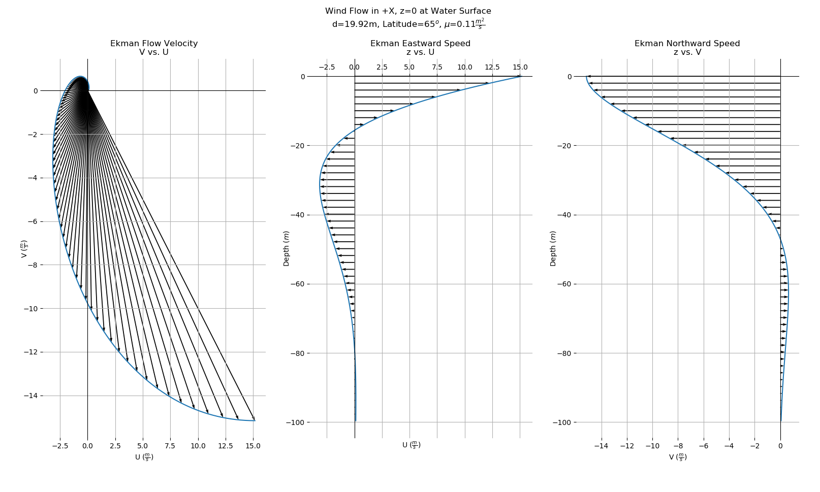
This result shows a surface flow 45$^\circ$. With a positive
(negative) signed f, the rotation will be to the right (left) in the
Northern (Southern) hemisphere. Next we can look at the net transport
across an entire Ekman layer. Integrating the velocity from the surface
to the infinitely deep bottom yields the net transport to be:
$\vec{U}_T = \int_{-\infty}^0
\left(\vec{u}
- \vec{\bar{u}} \right) dz = \int_{-\infty}^0 \left(
A(\delta)\mathbf{R}(\delta)\cdot\vec{\tau} \right) dz = d \cdot
\vec{\tau}\cdot \int_{-\infty}^0 \left(
A(\delta)\mathbf{R}(\delta) \right) d\delta $
The result of this integration can be shown to be:
$\vec{U}_T =\frac{1}{\rho_0 f}
\left[ {\begin{array}{cc}
0 & 1 \\
-1 & 0 \\
\end{array} } \right] \cdot \vec{\tau}$
The resultant rotation matrix is a 90$^\circ$ rotation to the right
(left) of the wind direction given a Northern (Southern) hemisphere
latitude and thus a positive (negative) sign of f. This behavior is
plotted below for an Eastward wind:
This view can, however, be misleading. A proper 3D view has been
plotted at the link below corresponding to the same initial conditions:
Super
Awesome 3D Plot of Ekman flow
Our model consists of a wind field over the Pacific ocean in the
Northern hemisphere. The grid is constrained to longitudes $\in\left[
180^\circ W,120^\circ W \right]$ and latitudes $\in\left[ 10^\circ
N,70^\circ N \right]$ with a resolution of $0.5^\circ$ in both
directions. We made a Gaussian style wind that exhibited both strong
divergence and curl, along with varying speed, with $0.5\%$ Gaussian
noise added. A 20$\frac{m}{s}$ max speed was applied to the Gaussian
wind profile and time steps were incremented with 3600$s$ resolution.
Ekman depth and f number were calculated at each grid element to
provide more authentic values. Finally ten surface buoys were placed in
the water and tracked for surface transport over time, they are
represented as diamonds on the plots. The data product we output has
four subplots: Upper Left (UL) showing wind and bulk transport, Upper
Right (UR) showing wind and surface transport, Lower Left (LL) showing
the vertical component of the curl of the wind, and Lower Right (LR)
showing the horizontal divergence of the wind field.

In the video version of this data product below you can see the bulk
transport (UL plot, calculated as above) is orthogonal to the wind, and
the surface speed of the water is 45$^\circ$ to the right (UR plot,
calculated as above).
Not
Quite as Awesome Ekman Transport Video