Artificial Life Part 3

3. The beginnings of a Boids model.

In order to begin designing the Boids model, it will be necessary to mathematically define the rules previously stated. Logically, it would be best to define the first rule.

1) Each creature must find a path from its starting point towards a goal, or perform an action to be determined by the animator.

In our case, the Boids will have no pre-defined goal, and will choose their own path. A coordinate system is set up:

R_{boid_N}(0) = ( X , Y , Z )

R_{boid_N}(T) = R_{boid_N}(0) + dR_{boid_N}(T)*T

If one is observant, it is easy to note that this is the parametric equation for a line describing the motion of a particle moving at a constant velocity. In the case of the real world, objects in motion rarely obey this equation over large time intervals of T, however, over an infinitesimally small time interval dT, one can approximate very complicated non-linear motions as being the sum of some arbitrary number of small linear motions.

This simple fact is the key to pulling off our simulation. We can now model the behavior of one Boid in space following only the first rule. Given a constant velocity, our Boid will follow a path from its starting point towards a goal: infinite T. Granted, it’s a simple goal, and a very uninteresting one at that, but one has to start somewhere, right?

Our second and third rules can be defined just as easily as the first.

2) A creature may not occupy space filled by an obstacle, and must maneuver to avoid them.

3) A creature may not occupy the space occupied by another creature and must maneuver to avoid collisions.

If we are to assume our Boids to have some unknown, arbitrary non-deformable shape, one can easily jump to a solution of simplifying each bid down to a sphere, or some other simple shape, with a maximum dimension that matches that of the bid. To test if one boid occupies the space of another, or that of an obstacle, assuming we treat each Boid as a sphere of radius r, simply measure the distance between each boid and make sure it is greater than two times the radius (Remember: each boid is a sphere of radius r) or simply the diameter of a single sphere:

R_N = ( X1 , Y1 , Z1 )

R_N-1= ( X2 , Y2 , Z2 )

Diameter D

Collision occurs if:

|| R_N-1- R_N || < D à (X2 - X1)² + (Y2 - Y1)² + (Z2 - Z1)² < D²

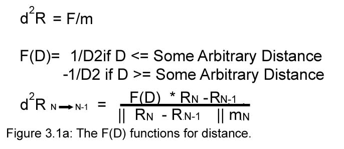
The first part of rules two and three have been defined, but how can the later parts be solved? This specific problem is a subject of much study, and there are many methods to do so. One of which is to give each Boid and object a vector force field of its own that varies with distance as in Figure 3.1a.

Suddenly, it’s easy to see that the above definition is a partial solution to the 4^th rule because the sum of each force vector, should (in theory) direct the boid towards the mean center of it’s peers.

4. If possible, a creature is to head towards the mean center of its peers within its range of perception.

It is a partial solution because “within its range of perception” has not been defined. To define what the range of perception entails, and why it is so important to our simulation requires a study of the vector field each boid generates. If we were to ignore the restriction put forward by the “range of perception”, we could assume that we were doing some sort of N-body attractions study--gravitational models, perhaps. Each Boid, while being counted as an unique particle, would have no say, as it were, in where it wished to moved. It would simply follow the rules of physics set down previously and “clump” together. Even with the added complication of the force direction changing sign below a certain distance, we could just assume they were gravitationally attracting balloons.

Now, suppose that some outside force gave all the boids uniform velocity. Then, suppose some immobile obstruction were placed in the path of this conglomeration of boid-particles. In theory, the conglomeration could “get stuck” around the obstruction with only the boids’ repulsion of the obstacle and mutual attraction at work.

Now, imagine the scenario where each boid is an “intelligent” particle, capable of selectively feeling an force from an obstacle or peer depending on the distance away it is. Now, only those boids a maximum distance away would be attracted to or repelled by the boid in question. Throw the boids towards an obstacle, and they will slip past it and congregate once more on the other side. Each boid cares only about it’s friends, or those that it can see, as it were. This behavior would seem to more closely model the behavior of real birds, which do not have to see the entire flock in order to successfully join it. It merely has to estimate the velocity and spacing of its closest neighbors to do so.

If a real bird behaved like a gravitational system, in the sense that they had to know the positions of each and every bird in their flock at all times to successfully choose their next movement, it would surely suffer from a mental break-down, after all, a real flock of birds can have hundreds, even thousands of birds in its ranks.

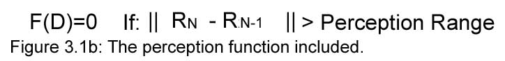
A simple method to model this perception would simply be to ignore any boids beyond a certain range, as in Figure 3.1b.

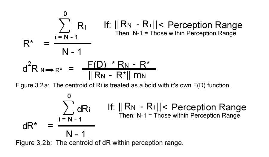A second method, which can also be used to solve the 5^th rule as well is to find the arithmetic average of each boid’s position or velocity vectors less than a certain distance away as in figure 3.2a:

So, rules one through five have been answered, but a number of implications produced by rules two through five have implications upon rule one, namely as each boid is now has an different and varying acceleration upon it, our standard definition for rule one cannot be used in its present state. If acceleration is no longer zero and no longer constant, then the motion of each boid is no longer necessarily linear. To more accurately model the boids over a large time-interval T would be very complicated, instead, we will again assume that we can only approximate the motion of the system over very small time intervals of T. Then, the equation put down in rule one need only be modified slightly to approximate the behavior as in figure 3.3.

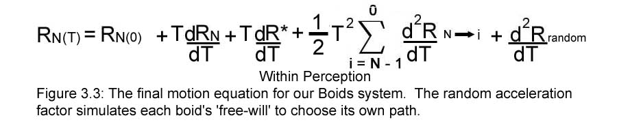
The equation has been modified such that over small T, acceleration (d²R) has been treated as a constant, the various velocities (dR) have also been treated as constant. In the equation in figure 3.3, an interesting term pops up involving a random acceleration vector. This random vector is used to represent each boid’s ‘free-will’: will the boid choose to peel away from the flock for whatever reason, or will it choose to stay with the group? Obviously, it would be difficult to model real bird psychology into this simple simulation, so a random number generator will suffice in generating enough randomness in the simulation to make things interesting at times.

Now, having defined all the parts of the simulation into a few simple equations, who wants a crack at simulating the behavior? Yes, you? Okay, here’s your pencil, and here’s your paper. Now, get cracking. One plus two plus five is eight...

Oh, that’s not what you had in mind, is it? You thought it would easier than this, did you? You thought that all we had to do was plug in a few numbers and this simple little equation would solve everything for you, did it? If you thought that, you are sadly mistaken, my friend. The fact of the matter is that the equation in figure 3.3 must be repeated many times before any hint of their significance can be seen. Even a slight change in the algorithm or the variables involved can have dramatic effects on the results. I’ve taken the liberty of programming a simple version of the simulation in a Java applet and provided the source code for download.

Despite the large number of similar and better simulations out there, I’m rather proud of my own simulation if I say so myself. The number of hours I put into making a working version of this simulation is significant; add to that the fact that I’m rather rusty in my programming skills, and it’s easy to understand why I nearly needed to change my drawers when I first clicked the run button on my compiler and saw these funny little dots dancing across the screen rather than the ubiquitous error messages that preceded them.

In this simulation, the Boids are constrained in a spherical universe of radius 250 units in which if they exceed the boundary, they re-enter the system on the opposite side with the same velocity. In addition, each time-frame represents 1/20th of a time-unit or iteration (which has no connection to any actual unit of time). I found this to give the best results animation-wise and helped to prevent the boids from jumping around across the screen without appearing to occupy the intervening space in-between. If one has a java-compiler of their own, feel free to twiddle with the various bits and pieces of my simulation and see how it effects the simulation. I lack the perseverance to design a working user-interface to make this simulation interactive, but I hopefully designed the base program well enough that anyone can find their way around in there once they set their minds to it.

Interested parties can get the source-code here:

Boids.java -- The applet interface, it would be wise not to twiddle too much here, it's easily broken.

Flock.java -- The guts of the simulation, fairly robust, with a number of methods() added that might have use in later versions.

VectorMathToolkit.java -- A separate class used to perform vector operations.

BACK